
Vector Database and how they can help you search unstructured data
Vector Databases can help you structure your unstructured data

In a previous post I’ve written about embeddings (Teaching a machine to read, how LLM's comprehend text). I strongly recommend reading that post before reading this, if you do not know what an embedding is. In short though, embeddings are a numerical representation of text, in the form of a vector (list of numbers).
Having and generating these embeddings are great. However if they are not stored somewhere, where they can be retrieved at a later time, they aren’t that useful. This is where we as a Data Engineers shine. We are great at putting stuff into databases.
Short comings of traditional relational databases
Before we try to use a new tool for solving a data storage problem, we should always check if we can solve our problem with a traditional relational database, like PostgreSQL, SQL Server or SQLite. These technologies are battle tested and readily available in most organisations.
However in the case of storing and retrieving embeddings these tools do have some limitations, which makes them unsuitable. Specifically retrieval performance is not up to par.
Traditional relational databases, are very good, when we want to retrieve a specific row (see row level storage part of Column Store Databases are awesome!). This however is not we need to in applications, where we use embeddings. What we need is something, which can retrieve the most similar embeddings in our database, based on a similarity score, such as cosine or dot product similarity.
Instead of thinking of our embedding as rows and columns, like we would with more traditional data. It makes more sense to look at them, as nodes in a graph, where similar embeddings are close to each other, and dissimilar embeddings are far from each other.

When we have a query, we do not necessarily want to find and exact occurrence instead what we want to do find the embeddings which are most similar to the query.

In our illustrations, we would want to extract the closest green embeddings.
A naive approach to doing this, would be to just compare vector similarity between our query, and all the embeddings in our database. We would then choose the top n most similar embeddings.
This could even work fairly well with a small enough dataset. The problem occurs when we have thousands or millions of embeddings. At this point, it is no longer a feasible task. We need to think about this in a different way, and this my friend is where vector databases comes into play. In the next sections, I'll help build your intuition around how they work.
Navigable Small World and 6 degrees of seperation
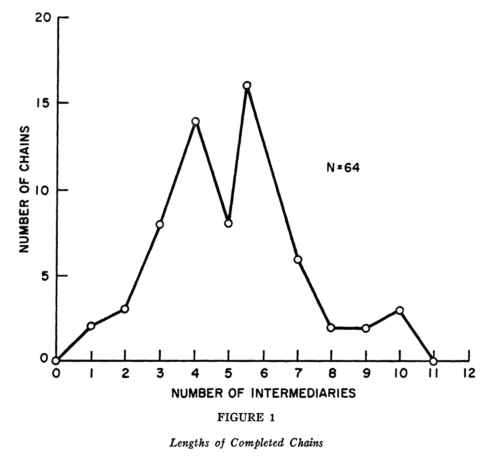
Six degrees of seperation is the idea, that you can reach just about any one in the world, going through chain of six people. This was explored empirically in Stanley Milgram’s An Experimental Study of the Small World Problem. In the experiment Milgram, would send a package to randomly selected people across the United States, and ask them to deliver the package to a specific person in Boston.
If they personally knew the person, they should send it to them directly, if not, they should send it to the person they knew, who were most likely to know the person.
These steps were then repeated for each package recipient, until the target person received the package.
Below are the number of intermediaries between the start and end from the original paper. As we can see most, packages were delivered using 6 intermediaries. Giving credence to the original six degrees of separation idea.
Dilovan you might ask, that’s all very interesting, but I’m trying to learn about vector databases, why are you talking about sending packages? To that I’ll answer hold your horses my friend.
Let’s try to visualise the network from the small world experiment in a different way. We can look at people as nodes in a graph, connected with other people via different social connections, and visualise these connections as edges.
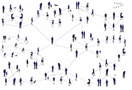
That looks a whole lot like the network graphs, we know from computer science.
Let’s say we would like to apply, what we’ve learned from the small world experiment to our problem of searching through embeddings.
First we would structure our data, so that the embeddings, are individual nodes in the network.
We then draw edges from each node, to the nodes which are similar to it. This type of graph, is called a Navigable Small World or NSW graph.
With our NSW graph, we can implement the search algorithm which Milgram used, in the following way.
Start with a random node in the network.
Move to the connected node, which are most similar to the target embedding.
Repeat until you cannot move to a new node which are more similar, than the one you are at.
Performing these steps, we should hopefully, end up in an area of our graph, where we can find the most similar embeddings to our query. We can then limit our search for the nearest embeddings to this area, instead of having to compare against all nodes in the network. In the graph from before, a search pattern could end up looking something like this.
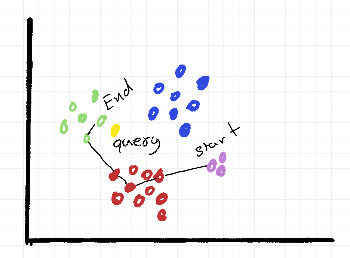
This is great, but our algorithm has 2 primary limitations. First, in a complex graph, the search can end up using a lot of steps, decreasing performance.
Second, the greedy search algorithm is prone to get stuck in a local optimum. Imagine we instead of traveling to the red cluster first, had travelled to the blue. If the blue, didn’t have a connection to the green cluster. We would be stuck the a local optimum in the blue cluster.
Hierarchical Navigable Small Worlds
To solve for these limitations Yu. A. Malkov and D. A. Yashunin published Efficient and robust approximate nearest neighbor search using Hierarchical Navigable Small World graphs. The paper proposes a layered approach to the Navigable Small World, which increases search speeds, and avoids getting stuck in local optimums.
It does so by creating different networks (layers), with varying edge length. The top layer having the longest edges and bottom the shortest.
If we look at our graph, we can quickly identify 4 different clusters (green, red, blue, magenta). The top layer might have one node from each of these clusters, and then a connection between each of these. The next layer would then hold the connections, between those nodes and the individual nodes in the cluster.
Starting our search at the top layer, ensures that we travel the appropriate cluster first. A greedy search algorithm is still used, but the layered approach addresses the short comings using an NSW graph.
The original paper, uses the following figure to illustrate the search.

Vector Databases and AI
Hierarchical Navigable Small World graphs (HNSW), is one of the techniques, which makes vector databases such a great choice for storing embeddings. But is not the only technique. Most vector databases, will implement a mix of different techniques. We might use PCA (Principal Component Analysis) or PQ (Product Quantisation), to reduce the dimensionality of the stored vectors and save on memory. We might even replace HNSW with IVF_FLAT, if you prioritise build time over read performance.
The point of this post is not necessarily to give you all the information, to implement your own vector database. Instead I hope you have a better understanding of how vector databases can work, and what it is they give us as data engineers. Whether you like it or not, AI is here to stay, and when using AI in your products, Vector Databases can be a very powerfull tool to have in your toolbox.
Let’s say you wanted to use a clustering algorithm to, categorise financial transactions, to build a fraud detection system. Using a vector database to store your output vectors, would greatly improve search performance as well as disk/memory requirements.
To get started with vector databases, you can use one of many the dedicated vector databases, such as Pinecone, Milvus and Chroma. Personally I’ve used the PostgreSQL extension pgvector, because it gives me the functionality I need, without the added complexity of adding a new database.